01. Intensity Gradient and Filtering

Locating Keypoints in an Image

As discussed in the previous lesson, a camera is not able to measure distance to an object directly. However, for our collision avoidance system, we can compute time-to-collision based on relative distance ratios on the image sensor instead. To do so, we need a set of locations on the image plane which can serve as stable anchors to compute relative distances between them. This section discussed how to locate such anchor locations - or keypoints in an image.

Take a look at the three patches in the following figure which have been extracted from an image of a highway driving scene. The grid shows the borders of individual pixels. How would you describe meaningful locations within those patches that could be used as keypoints?

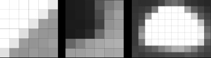
In the leftmost patch, there is a distinctive contrast between bright and dark pixels which resembles a line from the bottom-left to the upper-right. The patch in the middle resembles a corner formed by a group of very dark pixels in the upper-left. The rightmost patch looks like a bright blob that might be approximated by an ellipse.

In order to precisely locate a keypoint in an image, we need a way to assign them a unique coordinate in both x an y. Not all of the above patches lend themselves to this goal. Both the corner as well as the ellipse can be positioned accurately in x and y, the line in the leftmost image can not.

In the following, we will thus concentrate on detecting corners in an image. In a later section, we will also look at detector who are optimized for blob-like structures, such as the SIFT detector.

The Intensity Gradient

In the above examples, the contrast between neighboring pixels contains the information we need : In order to precisely locate e.g. the corner in the middle patch, we do not need to know its color but instead we require the color difference between the pixels that form the corner to be as high as possible. An ideal corner would consist of only black and white pixels.

The figure below shows the intensity profile of all pixels along the red line in the image as well as the intensity gradient, which is the derivative of image intensity.

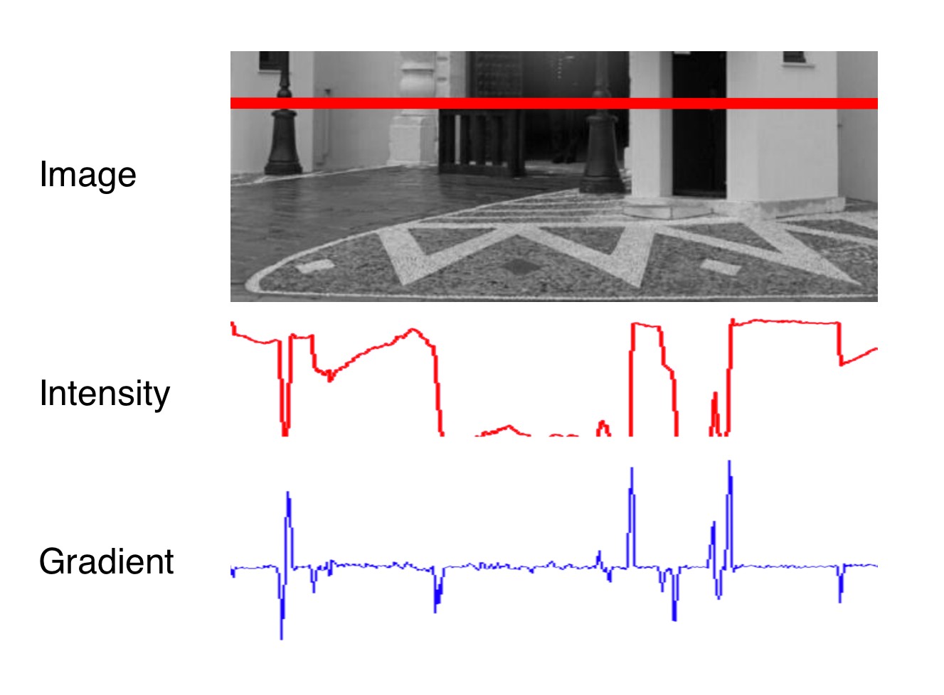
It can be seen that the intensity profile increases rapidly at positions where the contrast between neighboring pixels changes significantly. The lower part of the street lamp on the left side and the dark door show a distinct intensity difference to the light wall. If we wanted to assign unique coordinates to the pixels where the change occurs, we could do so by looking at the derivative of the intensity, which is the blue gradient profile you can see below the red line. Sudden changes in image intensity are clearly visible as distinct peaks and valleys in the gradient profile. If we were to look for such peaks not only from left to right but also from top to bottom, we could look for points which show a gradient peak both in horizontal and in vertical direction and choose them as keypoints with both x and y coordinates. In the example patches above, this would work best for the corner, whereas an edge-like structure would have more or less identical gradients at all positions with no clear peak in x and y.

Based on the above observations, the first step into keypoint detection is thus the computation of a gradient image. Mathematically, the gradient is the partial derivative of the image intensity into both x and y direction. The figure below shows the intensity gradient for three example patches. The gradient direction is represented by the arrow.

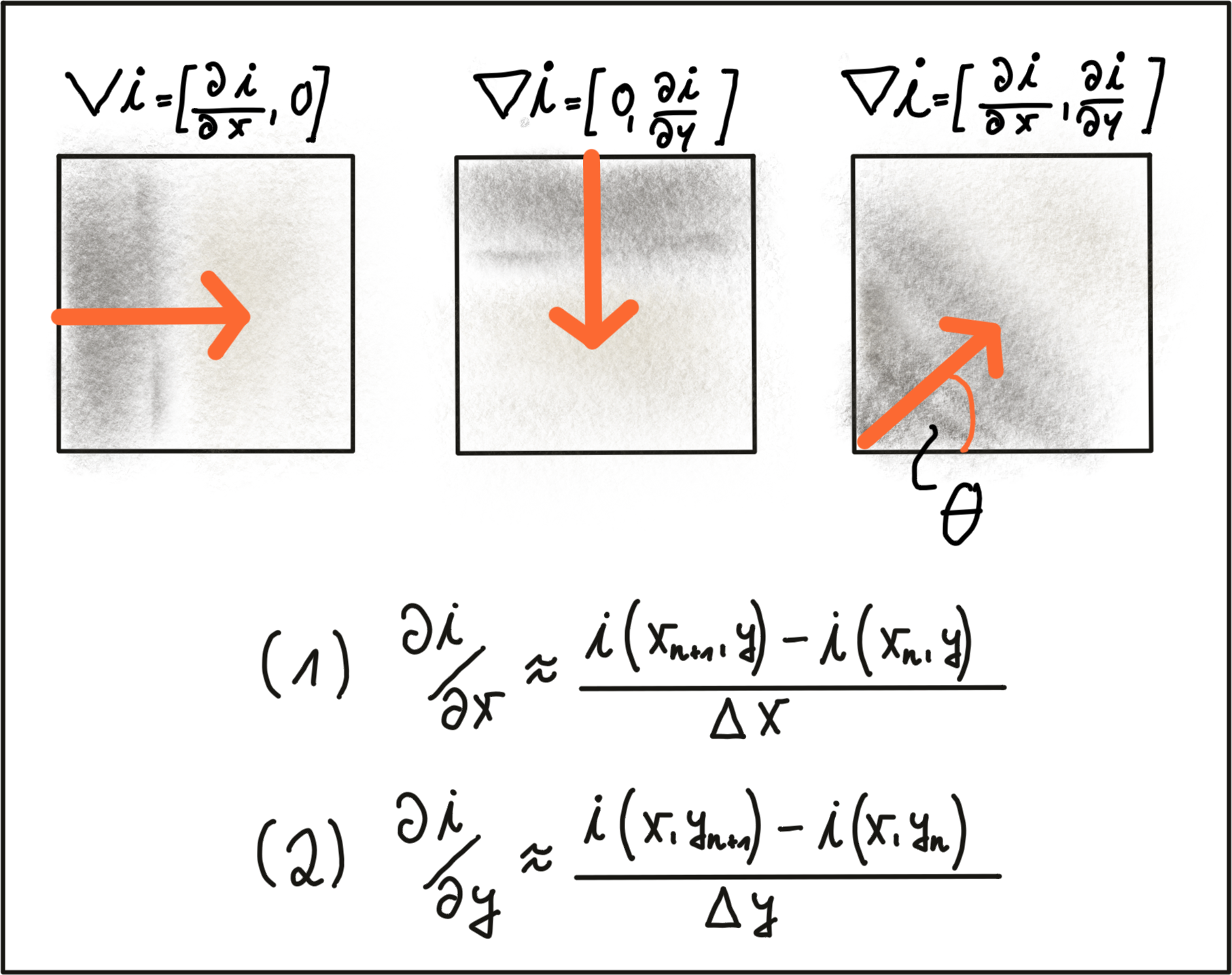
In equations (1) and (2), the intensity gradient is approximated by the intensity differences between neighboring pixels, divided by the distance between those pixels in x- and y-direction. Next, based on the intensity gradient vector, we can compute both the direction as well as the magnitude as given by the following equations:

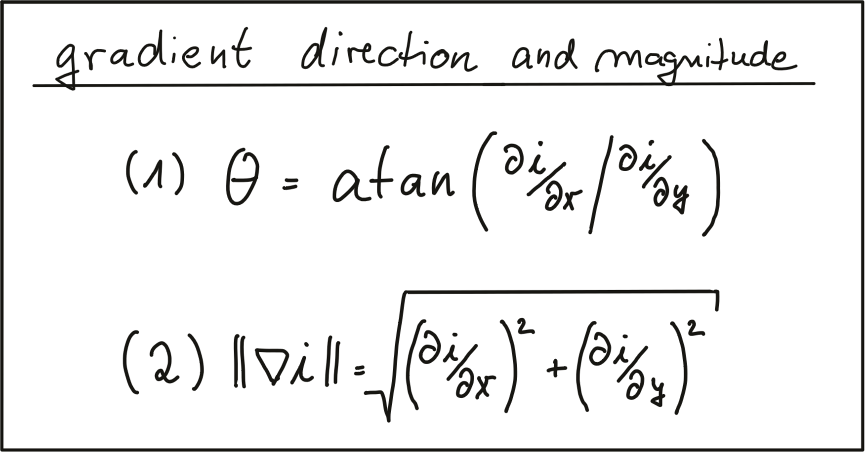
There are numerous ways of computing the intensity gradient. The most straightforward approach would be to simply compute the intensity difference between neighboring pixels. This approach however is extremely sensitive to noise and should be avoided in practice. Further down in this section, we will look at a well-proven standard approach, the Sobel operator.

Image Filters and Gaussian Smoothing

Before we further discuss gradient computation, we need to think about noise, which is present in all images (except artificial ones) and which decreases with increasing light intensity. To counteract noise, especially under low-light conditions, a smoothing operator has to be applied to the image before gradient computation. Usually, a Gaussian filter is used for this purpose which is shifted over the image and combined with the intensity values beneath it. In order to parameterize the filter properly, two parameters have to be adjusted:

1. The standard deviation, which controls the spatial extension of the filter in the image plane. The larger the standard deviation, the wider the area which is covered by the filter.
2. The kernel size, which defines how many pixels around the center location will contribute to the smoothing operation.

The following figure shows three Gaussian filter kernels with varying standard deviations.

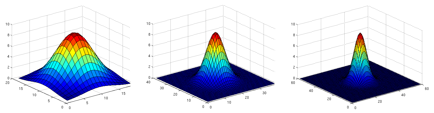
Gaussian smoothing works by assigning each pixel a weighted sum of the surrounding pixels based on the height of the Gaussian curve at each point. The largest contribution will come from the center pixel itself, whereas the contribution from the pixels surroundings will decrease depending on the height of the Gaussian curve and thus its standard deviation. It can easily be seen that the contribution of the surrounding pixels around the center location increases when the standard deviation is large (left image).

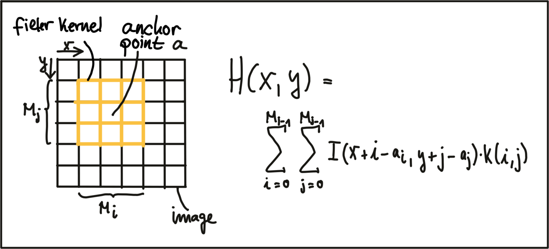
Applying the Gaussian filter (or any other filter) works in four successive steps which are illustrated by the figure below:

1. Create a filter kernel with the desired properties (e.g. Gaussian smoothing or edge detection)
2. Define the anchor point within the kernel (usually the center position) and place it on top of the first pixel of the image.
3. Compute the sum of the products of kernel coefficients with the corresponding image pixel values beneath.
4. Place the result to the location of the kernel anchor in the input image.
5. Repeat the process for all pixels over the entire image.

The following figure illustrates the process of shifting the (yellow) filter kernel over the image row by row and assigning the result of the two-dimensional sum H(x,y) to every pixel location.

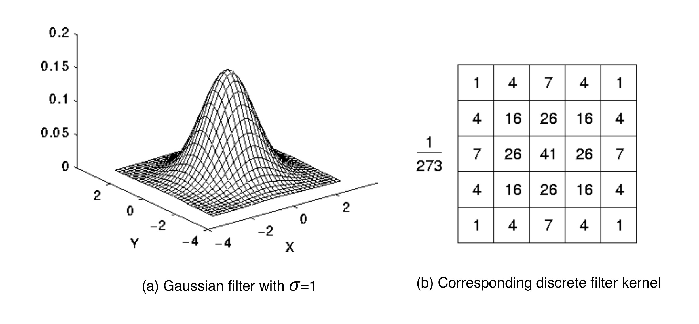
A filter kernel for Gaussian smoothing is shown in the next figure. In (a), a 3D Gaussian curve is shown and in (b), the corresponding discrete filter kernel can be seen with a central anchor point (41) corresponding to the maximum of the Gaussian curve and with decreasing values towards the edges in a (approximately) circular shape.

Exercise

The following code uses the function cv::filter2D to apply the filter above to an image. Run the code and figure out why the output image does not look as it is supposed to look after applying the smoothing filter. Once you know why, make the necessary changes and run the code again until you see a slightly blurred image. You can compile using cmake and make as before, and run the code using the generated gaussian_smoothing executable.

The above code is meant to illustrate the principle of filters and of Gaussian blurring. In your projects however, you can (and should) use the function cv::GaussianBlur, which lets you change the standard deviation easily without having to adjust the filter kernel.

Computing the Intensity Gradient

After smoothing the image slightly to reduce the influence of noise, we can now compute the intensity gradient of the image in both x and y direction. In the literature, there are several approaches to gradient computation to be found. Among the most famous it the Sobel operator (proposed in 1968), but there are several others, such as the Scharr operator, which is optimized for rotational symmetry.

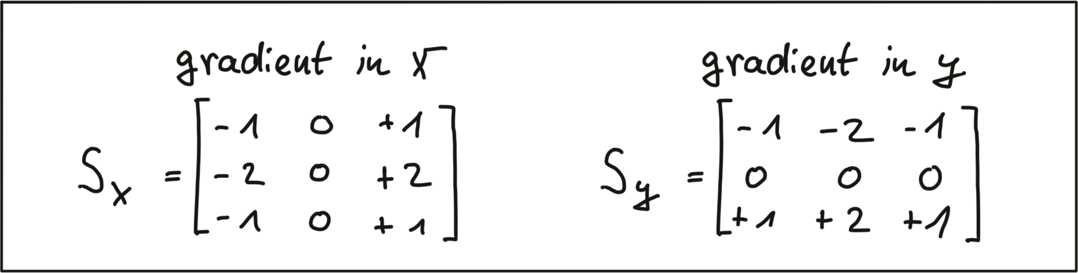
The Sobel operator is based on applying small integer-valued filters both in horizontal and vertical direction. The operators are 3x3 kernels, one for the gradient in x and one for the gradient in y. Both kernels are shown below.

In the following code, one kernel of the Sobel operator is applied to an image. Note that it has been converted to grayscale to avoid computing the operator on each color channel. This code can be found in the gradient_sobel.cpp file in the desktop workspace above. You can run the code by using the gradient_sobel executable.

    // load image from file
    cv::Mat img;
    img = cv::imread("./img1.png");

    // convert image to grayscale
    cv::Mat imgGray;
    cv::cvtColor(img, imgGray, cv::COLOR_BGR2GRAY);

    // create filter kernel
    float sobel_x[9] = {-1, 0, +1,
                        -2, 0, +2, 
                        -1, 0, +1};
    cv::Mat kernel_x = cv::Mat(3, 3, CV_32F, sobel_x);

    // apply filter
    cv::Mat result_x;
    cv::filter2D(imgGray, result_x, -1, kernel_x, cv::Point(-1, -1), 0, cv::BORDER_DEFAULT);

    // show result
    string windowName = "Sobel operator (x-direction)";
    cv::namedWindow( windowName, 1 ); // create window 
    cv::imshow(windowName, result_x);
    cv::waitKey(0); // wait for keyboard input before continuing

The resulting gradient image is shown below. It can be seen that areas of strong local contrast such as the cast shadow of the preceding vehicle leads to high values in the filtered image.

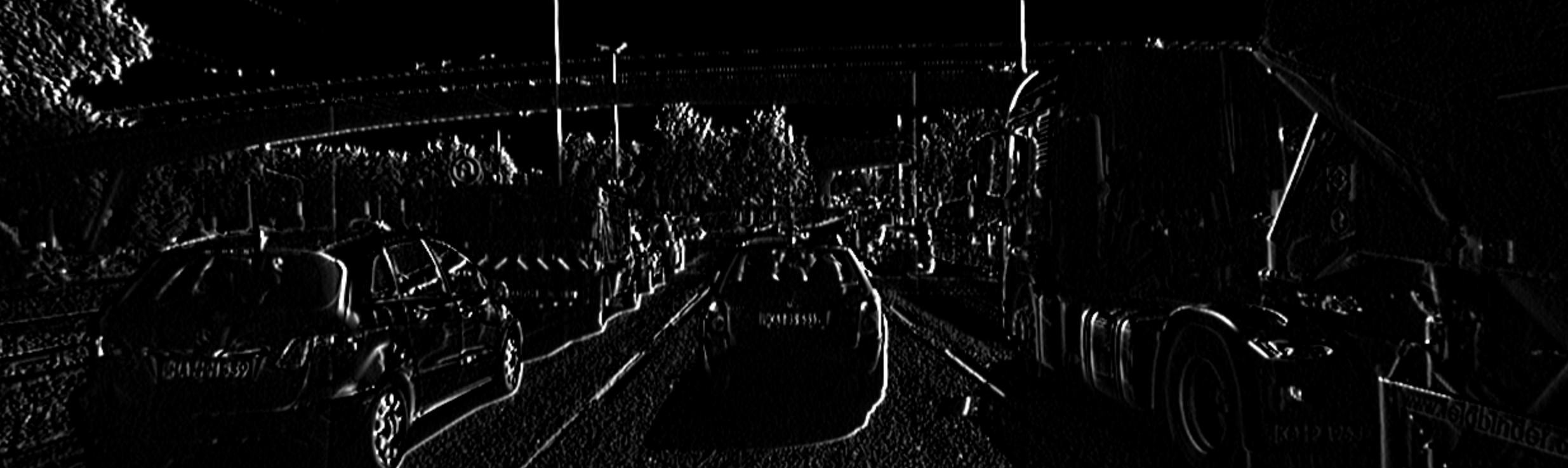
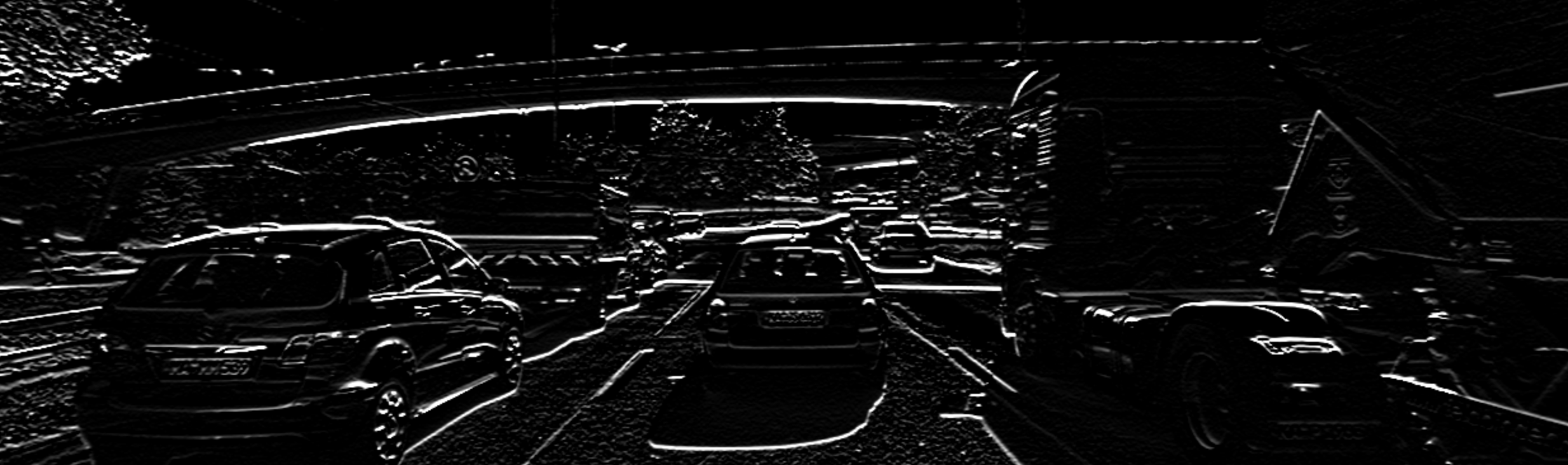
Note that in the above code, only the S_x filter kernel has been applied for now, which is why the cast shadow only shows in x direction. Applying S_y to the image yields the following result:

Exercise

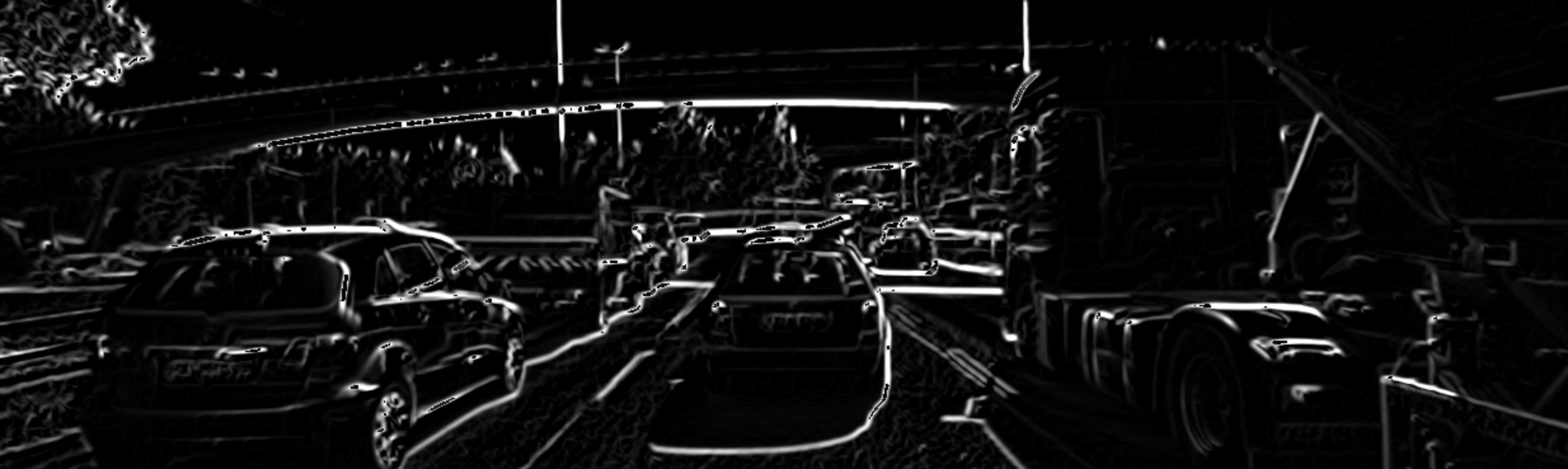
Based on the image gradients in both x and y, compute an image which contains the gradient magnitude according to the equation at the beginning of this section for every pixel position. Also, apply different levels of Gaussian blurring before applying the Sobel operator and compare the results.

You can use the magnitude_sobel.cpp file in the desktop workspace above for your solution, and after make , you can run the code using the magnitude_sobel executable.

The result should look something like this, with the noise in the road surface being almost gone due to smoothing: